In probability theory, the Kelly criterion, Kelly strategy Kelly formula, or Kelly bet, is a formula used to determine the optimal size of a series of bets. In most gambling scenarios, and some investing scenarios under some simplifying assumptions, the Kelly strategy will do better than any essentially different strategy in the long run. It was described by J. L. Kelly, Jr in 1956.[1] The practical use of the formula has been demonstrated.[2][3][4]
Although the Kelly strategy’s promise of doing better than any other strategy seems compelling, some economists have argued strenuously against it, mainly because an individual’s specific investing constraints may override the desire for optimal growth rate.[5] The conventional alternative is utility theory which says bets should be sized to maximize the expected utility of the outcome (to an individual with logarithmic utility, the Kelly bet maximizes utility, so there is no conflict). Even Kelly supporters usually argue for fractional Kelly (betting a fixed fraction of the amount recommended by Kelly) for a variety of practical reasons, such as wishing to reduce volatility, or protecting against non-deterministic errors in their advantage (edge) calculations.[6]
In recent years, Kelly has become a part of mainstream investment theory[7] and the claim has been made that well-known successful investors including Warren Buffett[8] and Bill Gross[9] use Kelly methods. William Poundstone wrote an extensive popular account of the history of Kelly betting.[5] But as Kelly’s original paper demonstrates, the criterion is only valid when the investment or “game” is played many times over, with the same probability of winning or losing each time, and the same payout ratio.[1]
Statement
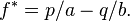
For simple bets with two outcomes, one involving losing the entire amount bet, and the other involving winning the bet amount multiplied by the payoff odds, the Kelly bet is:
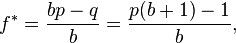
where:
- f* is the fraction of the current bankroll to wager;
- b is the net odds received on the wager (“b to 1″); that is, you could win $b (plus the $1 wagered) for a $1 bet
- p is the probability of winning;
- q is the probability of losing, which is 1 − p.
As an example, if a gamble has a 60% chance of winning (p = 0.60, q = 0.40), but the gambler receives 1-to-1 odds on a winning bet (b = 1), then the gambler should bet 20% of the bankroll at each opportunity (f* = 0.20), in order to maximize the long-run growth rate of the bankroll.
If the gambler has zero edge, i.e. if b = q / p, then the criterion recommends the gambler bets nothing. If the edge is negative (b < q / p) the formula gives a negative result, indicating that the gambler should take the other side of the bet. For example, in standard American roulette, the bettor is offered an even money payoff (b = 1) on red, when there are 18 red numbers and 20 non-red numbers on the wheel (p = 18/38). The Kelly bet is -1/19, meaning the gambler should bet one-nineteenth of the bankroll that red will not come up. Unfortunately, the casino doesn’t allow betting against red, so a Kelly gambler could not bet.
The top of the first fraction is the expected net winnings from a $1 bet, since the two outcomes are that you either win $b with probability p, or lose the $1 wagered, i.e. win $-1, with probability q. Hence:

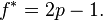
For even-money bets (i.e. when b = 1), the first formula can be simplified to:

Since q = 1-p, this simplifies further to
A more general problem relevant for investment decisions is the following:
1. The probability of success is  .
.
2. If you succeed, the value of your investment increases from  to
to  .
.
3. If you fail (for which the probability is  ) the value of your investment decreases from to
  . (Note that the previous description above assumes that a is 1).
In this case, the Kelly criterion turns out to be the relatively simple expression
Note that this reduces to the original expression for the special case above ( ) for
) for  .
.
Clearly, in order to decide in favor of investing at least a small amount  , you must have

which obviously is nothing more than the fact that your expected profit must exceed the expected loss for the investment to make any sense.
The general result clarifies why leveraging (taking a loan to invest) decreases the optimal fraction to be invested , as in that case  . Obviously, no matter how large the probability of success, , is, if
  is sufficiently large, the optimal fraction to invest is zero. Thus using too much margin is not a good investment strategy, no matter how good an investor you are.
Proof
Heuristic proofs of the Kelly criterion are straightforward.[10] For a symbolic verification with Python and SymPy one would set the derivative y'(x) of the expected value of the logarithmic bankroll y(x) to 0 and solve for x:
>>> from sympy import *
>>> x,b,p = symbols('xbp')
>>> y = p*log(1+b*x) + (1-p)*log(1-x)
>>> solve(diff(y,x), x)
[-(1 - p - b*p)/b]
For a rigorous and general proof, see Kelly’s original paper[1] or some of the other references listed below. Some corrections have been published.[11]
We give the following non-rigorous argument for the case b = 1 (a 50:50 “even money” bet) to show the general idea and provide some insights.[1]
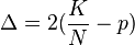
When b = 1, the Kelly bettor bets 2p – 1 times initial wealth, W, as shown above. If he wins, he has 2pW. If he loses, he has 2(1 – p)W. Suppose he makes N bets like this, and wins K of them. The order of the wins and losses doesn’t matter, he will have:

Suppose another bettor bets a different amount, (2p – 1 +  )W for some positive or negative . He will have (2p + )W after a win and [2(1 – p)- ]W after a loss. After the same wins and losses as the Kelly bettor, he will have:
![(2p+\Delta)^K[2(1-p)-\Delta]^{N-K}W \!](http://upload.wikimedia.org/math/a/4/b/a4b814d5ba30df6404506489e5905d33.png)
Take the derivative of this with respect to and get:
![K(2p+\Delta)^{K-1}[2(1-p)-\Delta]^{N-K}W-(N-K)(2p+\Delta)^K[2(1-p)-\Delta]^{N-K-1}W\!](http://upload.wikimedia.org/math/1/2/f/12f40e12d0632addfa09de7b4509b3c7.png)
The turning point of the original function occurs when this derivative equals zero, which occurs at:
![K[2(1-p)-\Delta]=(N-K)(2p+\Delta) \!](http://upload.wikimedia.org/math/d/3/8/d386e009e6ba02a60a46a9d992e43c64.png)
which implies:
but:
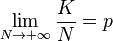
so in the long run, final wealth is maximized by setting to zero, which means following the Kelly strategy.
This illustrates that Kelly has both a deterministic and a stochastic component. If one knows K and N and wishes to pick a constant fraction of wealth to bet each time (otherwise one could cheat and, for example, bet zero after the Kth win knowing that the rest of the bets will lose), one will end up with the most money if one bets:
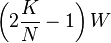
each time. This is true whether N is small or large. The “long run” part of Kelly is necessary because K is not known in advance, just that as N gets large, K will approach pN. Someone who bets more than Kelly can do better if K > pN for a stretch; someone who bets less than Kelly can do better if K < pN for a stretch, but in the long run, Kelly always wins.
The heuristic proof for the general case proceeds as follows.[citation needed]
In a single trial, if you invest the fraction  of your capital, if your strategy succeeds, your capital at the end of the trial increases by the factor
  , and, likewise, if the strategy fails, you end up having your capital decreased by the factor
  . Thus at the end of
  trials (with
  successes and
  failures ), the starting capital of $1 yields

Maximizing  , and consequently
  , with respect to leads to the desired result

For a more detailed discussion of this formula for the general case, see http://www.bjmath.com/bjmath/thorp/ch2.pdf.
Reasons to bet less than Kelly
A natural assumption is that taking more risk increases the probability of both very good and very bad outcomes. One of the most important ideas in Kelly is that betting more than the Kelly amount decreases the probability of very good results, while still increasing the probability of very bad results. Since in reality we seldom know the precise probabilities and payoffs, and since overbetting is worse than underbetting, it makes sense to err on the side of caution and bet less than the Kelly amount.
Kelly assumes sequential bets that are independent (later work generalizes to bets that have sufficient independence). That may be a good model for some gambling games, but generally does not apply in investing and other forms of risk-taking.
The Kelly property appears “in the long run” (that is, it is an asymptotic property). To a person, it matters whether the property emerges over a small number or a large number of bets. It makes sense to consider not just the long run, but where losing a bet might leave one in the short and medium term as well. A related point is that Kelly assumes the only important thing is long-term wealth. Most people also care about the path to get there. Kelly betting leads to highly volatile short-term outcomes which many people find unpleasant, even if they believe they will do well in the end.
The criterion assumes you know the true value of p, the probability of the winning. The formula tells you to bet a positive amount if p is greater than 1/(b+1). In many situations you cannot be sure p is the true probability. For example if you are told there are just 100 tickets ($1 each) to a raffle, and the prize for winning is $110, then Kelly will tell you to bet a positive fraction of your bank. However, if the information of “100 tickets” was a lie or mis-estimate, and if the true number of tickets was 120, then any bet needs to be avoided. Your optimal investement strategy will need to consider the statistical distribution for your estimate for p.
Bernoulli
In a 1738 article, Daniel Bernoulli suggested that when one has a choice of bets or investments that one should choose that with the highest geometric mean of outcomes. This is mathematically equivalent to the Kelly criterion[citation needed], although the motivation is entirely different (Bernoulli wanted to resolve the St. Petersburg paradox). The Bernoulli article was not translated into English until 1956,[12] but the work was well-known among mathematicians and economists.
Many horses[edit]
Kelly’s criterion may be generalized [13] on gambling on many mutually exclusive outcomes, like in horse races. Suppose there are several mutually exclusive outcomes. The probability that the k-th horse wins the race is  , the total amount of bets placed on k-th horse is
  , and
, and
where  are the pay-off odds.
  , is the dividend rate where
  is the track take or tax,
  is the revenue rate after deduction of the track take when k-th horse wins. The fraction of the bettor’s funds to bet on k-th horse is
  . Kelly’s criterion for gambling with multiple mutually exclusive outcomes gives an algorithm for finding the optimal set
  of outcomes on which it is reasonable to bet and it gives explicit formula for finding the optimal fractions
  of bettor’s wealth to be bet on the outcomes included in the optimal set . The algorithm for the optimal set of outcomes consists of four steps.[13]
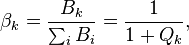
Step 1 Calculate the expected revenue rate for all possible (or only for several of the most promising) outcomes: 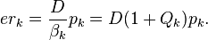
Step 2 Reorder the outcomes so that the new sequence  is non-increasing. Thus
  will be the best bet.
Step 3 Set  (the empty set),
  ,
,  . Thus the best bet
  will be considered first.
Step 4 Repeat:
If 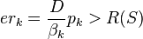 then insert k-th outcome into the set:
  , recalculate
  according to the formula:
 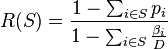 and then set
  ,
,
Else set  and then stop the repetition.
If the optimal set is empty then do not bet at all. If the set of optimal outcomes is not empty then the optimal fraction to bet on k-th outcome may be calculated from this formula:  .
.
One may prove[13] that
where the right hand-side is the reserve rate[clarification needed]. Therefore the requirement may be interpreted[13] as follows: k-th outcome is included in the set of optimal outcomes if and only if its expected revenue rate is greater than the reserve rate. The formula for the optimal fraction may be interpreted as the excess of the expected revenue rate of k-th horse over the reserve rate divided by the revenue after deduction of the track take when k-th horse wins or as the excess of the probability of k-th horse winning over the reserve rate divided by revenue after deduction of the track take when k-th horse wins. The binary growth exponent is

and the doubling time is

This method of selection of optimal bets may be applied also when probabilities are known only for several most promising outcomes, while the remaining outcomes have no chance to win. In this case it must be that  and
and  .
.
Application to the stock market
Consider a market with  correlated stocks
  with stochastic returns
  ,
,  and a riskless bond with return
  . An investor puts a fraction
  of his capital in and the rest is invested in bond. Without loss of generality assume that investor’s starting capital is equal to 1. According to Kelly criterion one should maximize
 ![\mathbb{E}\left[ \ln\left((1 + r) + \sum\limits_{k=1}^n u_k(r_k -r) \right) \right]](http://upload.wikimedia.org/math/6/d/e/6de30ae99c1da27e27e4ab92c95f7f79.png)
Expanding it to the Taylor series around  we obtain
![\mathbb{E} \left[ \ln(1+r) + \sum\limits_{k=1}^{n} \frac{u_k(r_k - r)}{1+r} -<br /><br /><br /><br /><br /><br /><br />
\frac{1}{2}\sum\limits_{k=1}^{n}\sum\limits_{j=1}^{n} u_k u_j \frac{(r_k<br /><br /><br /><br /><br /><br /><br />
-r)(r_j - r)}{(1+r)^2} \right]](http://upload.wikimedia.org/math/b/1/c/b1c2b08db45957bd88b0bdc60a5cb56c.png)
Thus we reduce the optimization problem to the Quadratic programming and the unconstrained solution is 
where  and
and  are the vector of means and the matrix of second mixed noncentral moments of the excess returns.[14] There are also numerical algorithms for the fractional Kelly strategies and for the optimal solution under no leverage and no short selling constraints.
See also[edit]
References
- ^ a b c d Kelly, J. L., Jr. (1956), “A New Interpretation of Information Rate”, Bell System Technical Journal 35: 917–926
- ^ Thorp, E. O. (January 1961), “Fortune’s Formula: The Game of Blackjack”, American Mathematical Society
- ^ Thorp, E. O. (1962), Beat the dealer: a winning strategy for the game of twenty-one. A scientific analysis of the world-wide game known variously as blackjack, twenty-one, vingt-et-un, pontoon or Van John, Blaisdell Pub. Co
- ^ Thorp, Edward O.; Kassouf, Sheen T. (1967), Beat the Market: A Scientific Stock Market System, Random House, ISBN 0-394-42439-5[page needed]
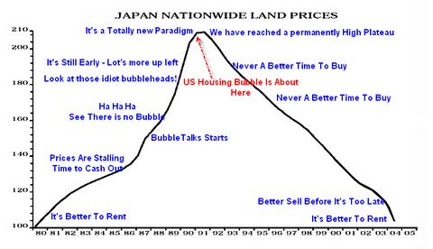
- ^ a b Poundstone, William (2005), Fortune’s Formula: The Untold Story of the Scientific Betting System That Beat the Casinos and Wall Street, New York: Hill and Wang, ISBN 0-8090-4637-7
- ^ Thorp, E. O. (May 2008), “The Kelly Criterion: Part I”, Wilmott Magazine
- ^ Zenios, S. A.; Ziemba, W. T. (2006), Handbook of Asset and Liability Management, North Holland, ISBN 978-0-444-50875-1
- ^ Pabrai, Mohnish (2007), The Dhandho Investor: The Low-Risk Value Method to High Returns, Wiley, ISBN 978-0-470-04389-9
- ^ Thorp, E. O. (September 2008), “The Kelly Criterion: Part II”, Wilmott Magazine
- ^ Press, WH; Teukolsky, SA; Vetterling, WT; Flannery, BP (2007), “Section 14.7 (Example 2.)”, Numerical Recipes: The Art of Scientific Computing (3rd ed.), New York: Cambridge University Press, ISBN 978-0-521-88068-8
- ^ Breiman, L. (1961) “Optimal Gambling Systems for Favorable Games”, Proc. Fourth Berkeley Symp. on Math. Statist. and Prob., Vol. 1 (Univ. of Calif. Press), 65-78. MR0135630
- ^ Bernoulli, Daniel (1956) [1738], “Exposition of a New Theory on the Measurement of Risk”, Econometrica (The Econometric Society) 22 (1): 22–36, JSTOR 1909829
- ^ a b c d Smoczynski, Peter; Tomkins, Dave (2010) “An explicit solution to the problem of optimizing the allocations of a bettor’s wealth when wagering on horse races”, Mathematical Scientist”, 35 (1), 10-17
- ^ Nekrasov, Vasily(2013) “Kelly Criterion for Multivariate Portfolios: A Model-Free Approach”


 1) “Fortune’s Formula” by William Poundstone